This clears out any previous lens data and prepares CODE V to define a new lens. A new lens "wizard" may be used to enter system design specifications, but let us suppose that we choose not to use the wizard. Instead, we enter the system data using the standard CODE V dialog boxes.
- Click
System SettingsA title is actually optional, but it's a good idea. The title appears on most graphical and tabular output.

Choose appropriate system units and enter your initials as the designer.
- Click
PupilCODE V needs to know the system aperture (or pupil size) of your system. This can be entered in one of four ways, entrance pupil diameter, numerical aperture at the object or image, or image space f/number; one of these must be entered, since there is no default pupil specifcation. The pupil specification defines the extent of the light bundles traced from each field point.

- Click
WavelengthsYou must specify at least one wavelength. An easy way to choose a number of wavelengths is to select a spectrum. We have chosen
Visible D. Wavelengths area always entered in nanometers, regardless of system dimensions.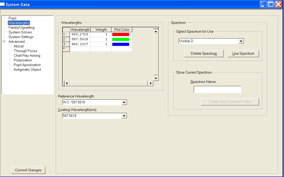
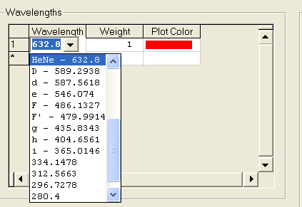
You may add or delete wavelengths from the list. Double-click the wavelength box to bring up a list of possible wavelength choices. You can change the weight and plot color associated with each wavelength as well.
- Click
Fields/VignettingMost systems have a non-zero field of view, and in CODE V we predefine one or more specfic field or object points at which to do analysis and optimization. For an infinite object distance, semi-field angle (in degrees) is the most common field specification.

Field angles should be entered in increasing order and should be entered as a Y-Angle for symmetric optical systems.
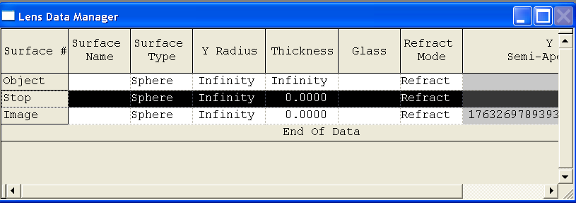
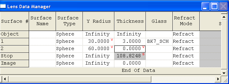
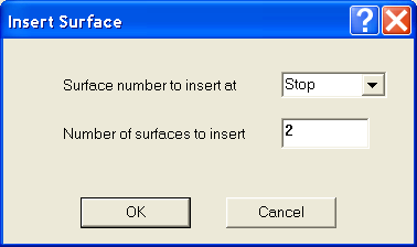
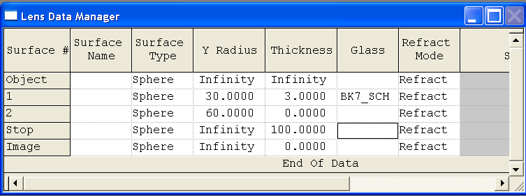
Right click on the Stop surface to bring up a context-sensitive menu. Choose Insert from that menu. This brings up the "Insert Surfaces" dialog. Insert two surfaces.
| Surface | Y Radius | Thickness | Glass |
|---|---|---|---|
| 1 | 30 | 3 | BK7 |
| 2 | 60 | 0 | |
| Stop | | 100 | |
You can double-click to highlight any field, then type a new value. You can also move between data fields with TAB (move right) and Shift-TAB (move left) keys, or move up and down with the vertical arrow keys or the up/down arrow toolbar buttons.

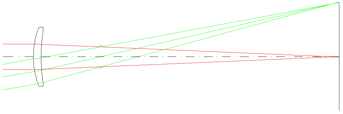
Now is a good time to draw a picture of the lens and verify that it looks reasonable. Plots are generated in a seperate plot window.
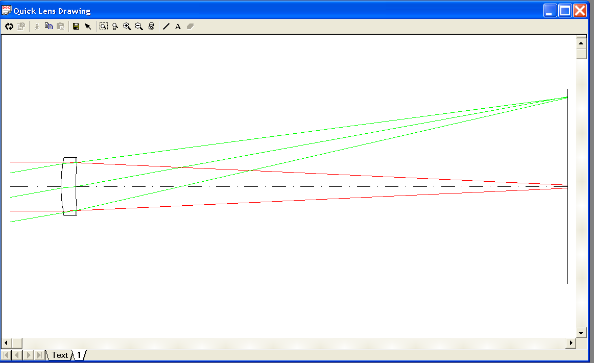
Notice how each field has a set of three rays displayed, the central ray and two marginal rays.
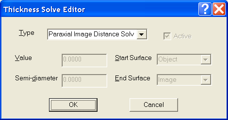
You may have noticed that the value of 100 mm was not a very good guess for the distance from surface 3 to the image. We could try various values to achieve better focus, but there's an easier way. The paraxial image solve can set the focal distance directly, without trial and error.
- Right click on the thickness of surface 3 (surface prior to the image surface)
- Menu: Solve
- Choose
Paraxial Image Distance Solveas the type of solve from the drop-down list box.
Note that after entering this solve the thickness is updated.
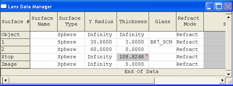
Furthermore, redrawing the lens (use the execute button  on the "Quick Lens Drawing" window) will show that the lens is now in focus.
We've done a fair amount of data entry, and the lens is a valid one (indicated by the prescence of non-blank first-order values on the bottom of the main Lens Data screen), so it would be wise to save our work in a disk file.