Resons

Example

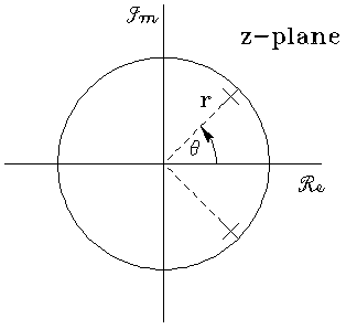
>> r = 0.996

r =

    0.9960

>> fs = 8192

fs =

        8192

>> [b,a] = reson(r,880/fs);
>> x = [1; zeros(4095,1)];
>> y = filter(b,a,x);
>> sound(y,fs)
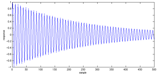
>> plot(0:500,y(1:501))
>> freqz(b,a)
>> y = y/max(abs(y));
>> wavwrite(y,fs,'reson.wav');
>> sound(y)
>> N=500;
>> plot(0:N,y(1:N+1));
>> xlabel 'sample'
>> ylabel 'response'

Matlab code for a Reson

function [b,a] = RESON(rho,theta)
%  RESON
%
%    Reson filter
%
%        RESON(rho,theta)
%

re = rho*cos(2*pi*theta);
si = sin(2*pi*theta);
b = (1-rho^2)*si;
a = [1 -2*re rho*rho];

Reson with DC-suppression

Add a zero at +1 to suppress the DC gain. This improves the low-frequency fall-off at the expense of the high-frequency fall-off. This example is centered at 15 Hz with a bandwidth of 5 Hz, sampled at 8 kHz. The blue curve shows the response without the zero, and the black curve shows the response with the zero.

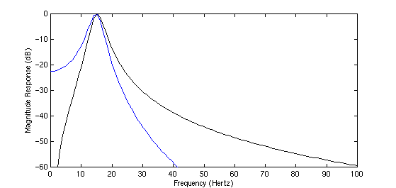
>> fs = 8000;
>> b = 2*pi*5/8000

b = 

    0.0039

>> r = exp(-b/2)

r =

    0.9980

>> theta = 15/8000

theta =

    0.0019

>> [b,a] = reson(r,theta);
>> h1 = freqz(b,a,f,fs);
>> b2 = [b -b];
>> h2 = freqz(b2,a,f,fs);
>> b2 = b2/max(abs(h2))
>> h2 = freqz(b2,a,f,fs);
>> plot(f,20*log(abs(h1)));
>> hold
Current plot held
>> plot(f,20*log(abs(h2)),'k');

Warning: Log of zero.
>> axis([0 100 -60 0])
>> ylabel 'Magnitude Response (dB)'
>> xlabel 'Frequency (Hertz)'

Equalizer Filter

Another slight generalization of the reson is to place a pair of zeros near the poles along the same direction as the poles. The poles are a distance ra from the origin and the zeros at a distance rb. In the figure below the zeros and poles are very close together and very close to the unit circle.

When the pole and zero are very near each other, the frequency response remains essentially flat for frequencies far from the resonant frequency. Near the pole/zero pair, the frequency response will rise if the peak is closer to the unit circle or fall if the zero is closer to the unit circle.

boost filter

notch filter

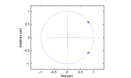
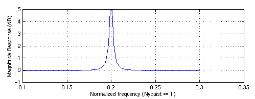
>> ra = 0.995
>> rb = 0.990
>> theta = 2*pi/10;
>> b = [1 -2*rb*cos(theta) rb*rb];
>> a = [1 -2*ra*cos(theta) ra*ra];
>> w = linspace(0.1,0.3,100);
>> freqz(b,a,w*pi); % boost filter
>> freqz(a,b,w*pi); % notch filter

Maintained by John Loomis, last updated 6 Nov 1997