Linear Search Example

dx3.m

global cv th rn;
cv = [ 0 0.25 -0.15];
th = [ 0  0    0];
rn = [ 1 1.5 1 ];

x = [ 0.25 -0.15]';
for (k=1:2)
   [A fz] = calculate_derivatives(@sing2,x);   
   s = -A\fz;
   x = x + s;
end
[A fz] = calculate_derivatives(@sing2,x);
s = -A\fz;

p = linspace(0,3,101);
for (k=1:101)
    f = fz + A*(p(k)*s);
    fig1(k)=norm(f);
    f = sing2(x+p(k)*s);
    fig2(k)=norm(f);
end

idx=find(fig1<0.025);

plot(p(idx),fig1(idx),p,fig2);
xlabel('p');
ylabel('\s');

Output

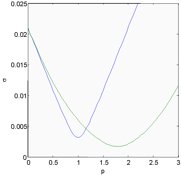
The array fig1 (s₁, in blue) is the norm of the linear defect model as a function of parametric distance along the solution vector.

The array fig2 (s₂, in green) is the norm of the actual defect function versus the parametric distance along the solution vector.

The plot suggests that the linear defect model applies only in a relatively small region near the starting point, at least far away from the actual solution.

Maintained by John Loomis, last updated 6 Feb 2003