2D Discrete Fourier Transform

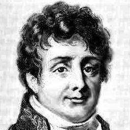
Fourier (1768 - 1830)	Fourier's transform

Steps in generating a Fourier transform image.

Files used in this study may be downloaded from: happyface.zip.

image	description	source code
	Start with a simple piece of artwork (55 x 55). smile = imread('smile.tif');	smile.tif
	Embed it in a 64 x 64 array. smile1 = fftprep(smile);	fftprep.m
	Reduce the size to keep our images small (optional). smile2 = reduce(smile1);	reduce.m
	Embed this image in a 128 x 128 array (larger size optional). smile_embed = fftprep(smile2,128);	fftprep.m
	Remap the origin to the upper left corner smile_embed = fftshift(smile_embed);	fftshift.m
complex-valued image	Run the Fourier transform program. smile_fft = fft2(smile_embed);	fft2.m
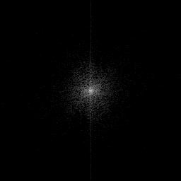
	Construct the square modulus = (real*real+imag*imag), scale the results to a maximum value of unity, and remap the origin back to the center of the image. sqmod = smile_fft.*conj(smile_fft); sqmod = fftshift(sqmod)/max(sqmod(:));
	Use logarithmic enhancement to see details. The default stretches 4 decades of values. out = logim(sqmod);	logim.m

A simple example

Before applying the Fourier Transform to general images, we really should apply it to a case for which we know the answer.

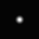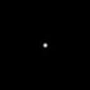
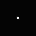
The input image is a circular disk with a radius of 4 pixels centered in a 128 x 128 array. The output image is the square modulus of the resulting Fourier transform. A cross-section of the output image is shown below.

The marked data points are taken from a horizontal cross-section of the output image. The solid curve is the ideal function, which was generated from somb(r/16).^2 (source code: somb.m). The factor of 16 converts pixel distance to the appropriate normalized distance.

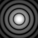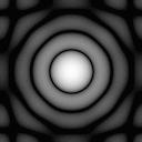
FFT	ideal result

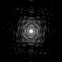
The image on the left is a logarithmic transformation of the output image, and shows the Airy rings. Note the departure from circular symmetry at the outskirts of the image. These artifacts are due to sampling the input function onto a rectangular grid. The artefacts are exaggerated by the logarithmic transformation.

The image on the right was generated from the ideal analytic function somb(r/16).^2 and demonstrates the correct visual appearance.

Maintained by John Loomis, last updated 8 March 2000