Gradient Filters

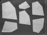
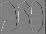
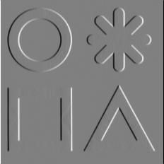
original image	x-gradient	y-gradient

Definition of the gradient operator

The gradient of a function is defined as

There are two components of a gradient image, the x-gradient and the y-gradient .

Finite-difference formulas for first derivative

The simplest approximation to the first derivative is the forward difference:

There is a similar backward difference formula.

The following two formulas are central difference formulas

The first central difference formula can be interpreted as the average of the simple forward difference and backward difference formulas.

First-derivative filter

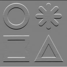
The simple forward difference formula is expressed as a convolution filter.

The forward and backward difference formulas reduce to the same 1 x 2 matrix (although the implementation is different).

Example of simple forward difference filter

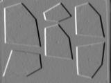
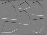original image	x-diff	y-diff

Bipolar images

Gradient filters can produce either positive or negative pixel values (z values). Images with negative z values are called bipolar images. Ordinary images have z values ranging from 0 to 1 (or 0 to 255 for common byte-oriented systems). Since only ordinary images can be displayed, one may ask how bipolar images should be displayed. The answer is to use pseudo coloring.

The scheme used here is to define bipolar images to be normalized such that |z| varies between 0 to to 1. Then the pixel transformation z' = 0.5 * z + 0.5 is applied. The zero level is mapped to mid-gray. Negative values are darker, with a maximum limit of black. Positive values are brighter, with a maximum limit of white.

The light regions in the gradient images above indicate a positive gradient (from darker to lighter in the original image). The dark regions indicated a negative gradient (from lighter to darker).

Smoothed gradient filters

The gradient operator is often combined with a smoothing filter, since numerical differentiation is a noise amplifying process.

Matlab example

original image	x-gradient
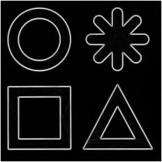y-gradient	gradient magnitude

» g = imread('half_target.tif');
» g = im2double(g);
» h = [ 1 2 1; 0 0 0; -1 -2 -1]

h =

     1     2     1
     0     0     0
    -1    -2    -1

» gy = filter2(h,g);
» max(max(gy))

ans =

    3.9373

» min(min(gy))

ans =

   -3.9098

» gyview = (gy+4)/8;
» -h'

ans =

    -1     0     1
    -2     0     2
    -1     0     1

» gx = filter2(-h',g);
» gxview = (gx+4)/8;
» imshow(gxview)
» imwrite(gxview,'gx.jpg');
» imwrite(gyview,'gy.jpg');
» gnorm = sqrt(gx.*gx+gy.*gy);
» max(max(gnorm))

ans =

    4.1706

» gnormview = gnorm/max(max(gnorm));
» imshow(gnormview);
» imwrite(gnormview,'gn.jpg');
» imwrite(g,'g.jpg');

Maintained by John Loomis, last updated 2 March 2000