
The equation of a plane is

We seek to find the best-fitting plane to a local 3 x 3 area of an image. The elements of the image Z in that neighborhood are shown below
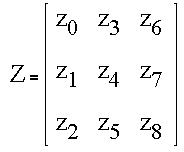
The array can be converted to a column vector by numbering the elements as shown. In Matlab, this would be equivalent to the operation Z(:).
Next we define arrays containing the local values of x and y over the neighborhood. We assume that the center pixel is the origin and that x increases to the right and y upward.

These arrays can also be converted to column vectors, as shown below.
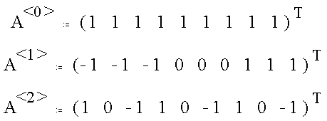
We have encountered these masks before and have noted their orthogonality. In this context, the expression of orthogonality is as follows. Note that the multiplications are really dot products.

We can generate a "covariance matrix" C that summarizes all combinations of the dot products.
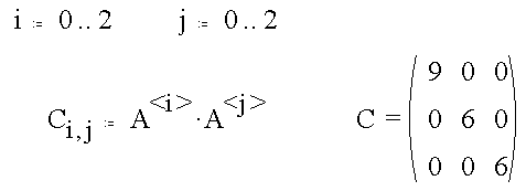
In the method of least squares, the unknown coefficients are chosen to minimize the mean square deviation of the image values from the fitted plane.

The values of the coefficients are found by setting the derivative with respect to each coefficient to zero and then solving the resulting set of equations for the coefficients.

The derivatives are given by the following equation

which can be simplified by using dot-product notation

Since the columns of the A matrix are orthogonal, the general solution reduces to
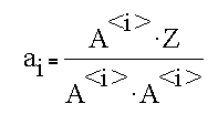
The explicit solution, obtained by evaluating the denominator, is given by
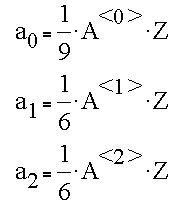
We define the location of an edge as the line of intersection between the plane and the midpoint gray value between the high and low border plateaus.

The equation for this line is

Suppose we have a portion of an image as follows
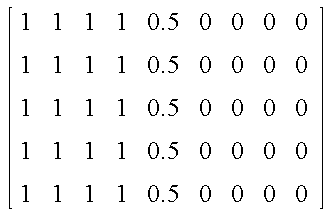
This is a vertically oriented edge such that

Furthermore, the height of the edge is 1, so the midpoint is located at

The the location of the edge in the x-direction (relative to the central pixel) can be found from

Suppose we evaluate the edge location at several positions.
The neighborhood at the center of the edge is
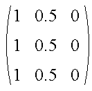
The associated Z vector is given by

and the least-squares values for the coefficients of the plane are

The equation of the plane can then be written as

The edge center is obtained by solving for the intersection of the plane with the edge midpoint.

This solution yields

which is the expected result.
The neighborhood one pixel to the left of the center of the edge is
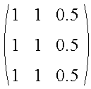
The associated Z vector is given by

and the least-squares values for the coefficients of the plane are

The equation of the plane can then be written as

The edge center is obtained by solving for the intersection of the plane with the edge midpoint.

This solution yields

which is not the expected result (x=1). The projection is wrong because we are on the shoulder of the edge rather than the planar ramp. The calculation does suggest that edge center is inside the next pixel to the right.
The neighborhood one pixel to the right of the center of the edge is
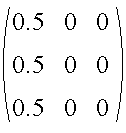
The equation to be solved for the edge location is

This solution yields

which again is not the expected result (x=-1), but does indicate that the edge lies in the pixel to the left.
The matrix below shows a sharp edge transition from 1 to 0
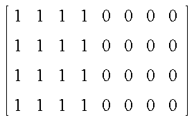
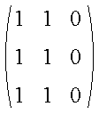
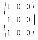
Using the equations for a plane and an edge midpoint of z = 0.5 gives the following results
| Neighborhood | Calculated location | Expected location |
|---|---|---|
 |  |  |
 |  |  |
The algorithm for finding edges, as developed so far, works if the edge is broad enough but is not exact for sharp edges. We can correct this situation by introducing a external weighting function.
The equation for weighted least-squares is

The coefficients of the plane are found as before, and are given by
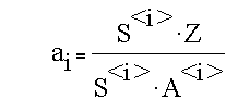
where

The appropriate weights are found in the following linear example.
In one-dimension, we have the following equation for the edge ramp.

A general weighted set of masks (given the need for symmetry) is

For these masks the coefficients are given by

Pixel values in the neighborhood of a sharp edge are given by

The cofficients are then

The edge location is given by the following equation

We can substitute the known values for the midpoint (z_m = 0.5) and edge location (x=0.5)

The solution to this equation is

In two dimensions the weight array can be constructed from
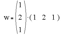
and expressed either as

The resulting masks are given by

The last two expressions are the familiar Sobel operators.
Orthogonality and variance values are obtained from

and the least-squares values for the plane coefficients are given by

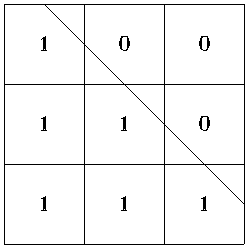
Consider the following skew edge
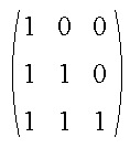
The pixel array is expressed as

The mask operators are expressed as
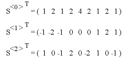
The equations for the coefficients are

and the coefficients themselves are

The equation for the edge location is given by

The edge is shown in the following diagram
Maintained by John Loomis, last updated July 11, 1997