Color Edges

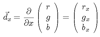
Form the spatial derivatives of the color vector, yielding the color derivative vectors:

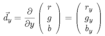
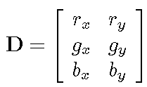
Assemble the derivative vectors into a single (3 x 2) spatial derivative matrix:

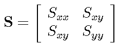
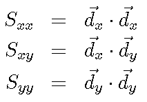
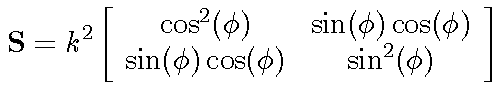
Take the "magnitude" of the spatial derivative matrix to form the matrix S

The matrix S is a (2 x 3)(3 x 2) = (2 x 2) matrix whose elements can be defined as follows:

Effect of Rotation Transformation on S

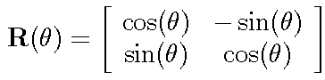
Rotate the coordinate axes by an angle q and calculate S' in the new coordinate system. The rotation transformation matrix is R(q):

The transformed spatial derivative matrix D' is given by:

and S' is then given by

Monochromatic (grayscale) edge orientation

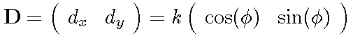
In the case of monochromatic images, the spatial derivative matrix can be written as

The rotated spatial derivative matrix is then

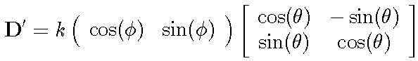
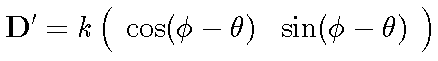
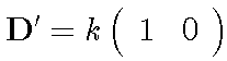
It is easy to see that a rotation of q = f aligns the x-axis with the direction of D and the transformed matrix D' has the following simple form

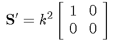
and the matrix S' is diagonalized, with eigenvalues of k² and 0.

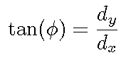
The edge orientation, for monochromatic edges, can be found directly from the spatial derivative matrix as

Edge orientation can also be found from the S matrix

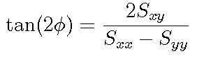
In this latter case, the orientation angle 2f, is found rather than the angle f directly. The significance of this is that finding f allows us to distinguish between f = 0 (a right directed edge) and f = p (a left directed edge). By finding 2f we lose the ability to distinguish right-directed from left-directed because the tan(2f) is the same in either case. The situation is analogous to taking the square of a scalar and thereby losing the sign of the scalar.

Color edge orientation

In the case of color edges, the matrix element S'_xy in the rotated coordinate system is given by

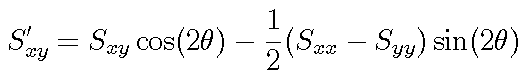
This off-diagonal element can be set to zero by choosing q to satisfy

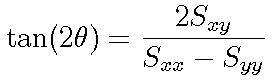
The diagonal elements in the rotated coordinate system are given by

Notice from the above equations that the trace of the matrix S is the same before and after any rotation.

Example 1, blue-red ramp

In the above ramp, S_xy = S_yy = 0, and the ramp is horizontally aligned. The question of increasing or decreasing has no meaning in this context. We can speak only of the horizontal orientation of the ramp.

Making the ramp

» x = linspace(0,1,101);
» x = ones(24,1)*x;
» ramp = cat(3,x,zeros(size(x)),1-x);
» imwrite(ramp,'blue-red.tif');

The element S_xx = 8e-4. The slope is 0.01 per pixel for red and blue. The Sobel operator magnifies the slope by 2, and S is proportional to the square of the slope.

Example 2, Color Triangle

This example illustrates an image which has a non-zero trace, but no preferred direction (except at the boundaries).

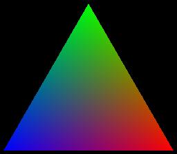
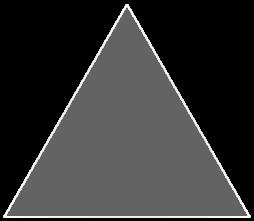
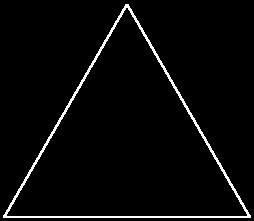
The image and its edge components are found first.

» tri = tri1(256);
» imshow(tri);
» [sxx,sxy,syy] = color_edge(tri);

Plots of S_xx-S_yy and 2 S_xy show large non-zero values only at the boundaries.

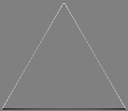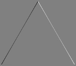Sxx-Syy	2 Sxy

» diff1 = imdiff(sxx,syy);
maximum difference: 0.990638
» imwrite(diff1,'tri-diff1.jpg');
» diff2 = imdiff(2*sxy);
maximum difference: 1.11574
» imwrite(diff2,'tri-diff2.jpg');

A plot of the trace S_xx+S_yy shows that there is a color gradient in the interior of the triangle.

» gz = sxx + syy;
» trace = logim(gz,6);
» imwrite(trace,'tri-trace.jpg');
» gz(128,128)

ans =

  2.6614e-004

Calculating the ratio of the directed edge gradient gn to the undirected edge gradient gz allows us to display the relative magnitude of the directed edge gradient.

» gx = sxx - syy;
» gy = 2*sxy;
» gz = sxx + syy;
» gn = sqrt(gx.*gx+gy.*gy);
» ga = 0.5*atan2(gy,gx);
» ratio = zeros(size(gz));
» idx = find(gz>0);
» ratio(idx) = gn(idx)./gz(idx);
» log_ratio = logim(ratio,6);
» imwrite(log_ratio,'tri-ratio.jpg');

Example 3, Color Image

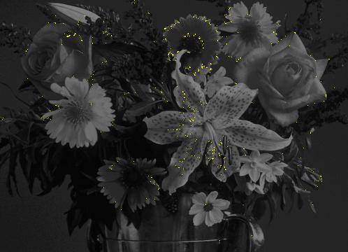
Ordinary color images generally have strongly oriented edges.

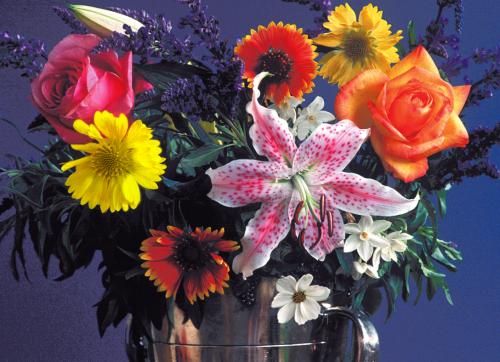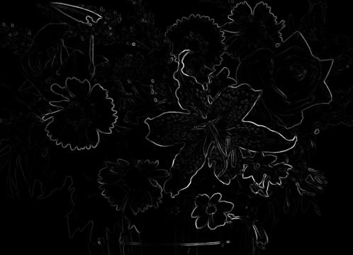input image	directed edge magnitude

» rgb = imread('flowers.tif');
» [sxx, sxy, syy] = color_edge(rgb);
» imwrite(rgb,'flowers.jpg');
» gx = sxx - syy;
» gy = 2*sxy;
» gz = sxx + syy;
» gn = sqrt(gx.*gx+gy.*gy);
» ga = 0.5*atan2(gy,gx);
» imwrite(imdiff(gn),'flowers_gn.jpg');
maximum difference: 2.31262

The image on the left below shows as white regions where the edge magnitude is large (gz > 0.1). The image on the right below shows as white regions where the directed edge magnitude (gn) is small compared to the relatively large total edge magnitude (gz). Very little area of the image contains undirected color edges.

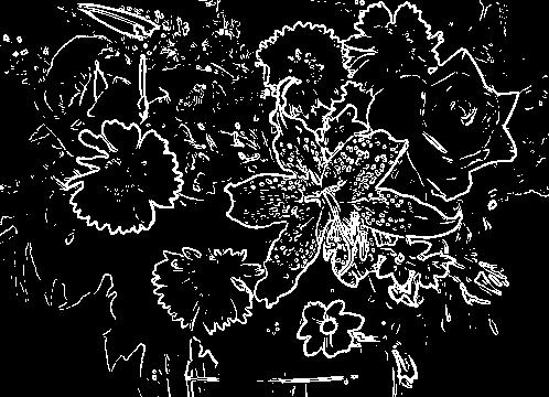gz > 0.1	(1 - gn/gz) > 0.2

» gt = gz>0.1;
» imwrite(gt,'flowers_gt.jpg');
» ratio = zeros(size(gz));
» idx = find(gt);
» ratio(idx)=1-gn(idx)./gz(idx);
» imwrite(ratio,'flowers_ratio.jpg');
» gray = rgb2gray(rgb);
» gray = im2double(gray);
» h = [ 0 0 0; 0 1 0; 0 0 0];
» g = filter2(h,gray,'valid');
» gmsk = g.*(ratio<0.2);
» bmsk = (ratio>=0.2);
» diff = cat(3,0.5*gmsk+bmsk,0.5*gmsk+bmsk,0.5*gmsk);
» imwrite(diff,'flowers_ratio_gtpt2.jpg');