The image source used is the Cleveland Browns Construction Cam. This internet camera was positioned to monitor the construction of the new Browns' Stadium. This camera is unique because of the following characteristics:
Ten pictures were captured for this analysis.

The images are loaded into MatLab using base.m. Throughout the following operations, care must be exercised to minimize the memory used in MatLab. This is accomplished by converting the images to and from DOUBLE and UINT8 types. The UINT8 type requires significantly less memory for each image than DOUBLE.
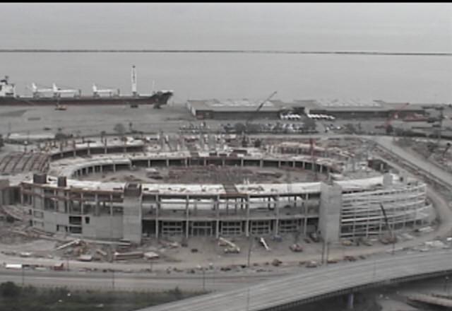
The horizontal bands running through the image are typical of NTSC camera images. This type of noise is the result of aliasing between the 60Hz refresh rate of the camera and the 60Hz power line frequency used in the United States. This is corrected by averaging all the frames together and calculating an average RBG pixel value for each scan line. This average is then used to scale each individual scan line of each picture to match. The MatLab file that performs this operation is hhist.m. A copy of the average picture is at the top of the page. Note: my copy of hhist.m was written with out reference to or knowledge of the MatLab Image Processing Tool box function of the same name and approximate function.

Once corrected for power supply noise, the images are saved using saveimg.m.
Each corrected image is then compared with the average image to locate differences. The identified differences are then expanded using filter2 to produce enlarged areas of differences. Finally, a "clean" image is created by averaging all ten images again. However, this time the portions of each image in the identified difference areas are excluded and do not contribute to the average. These operations are performed by mask.m and combine.m. The combined "clean" image is at the top of the page. The final output is generated using output.m.
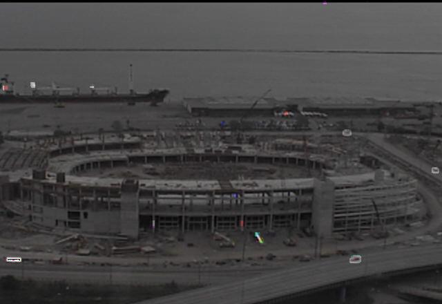
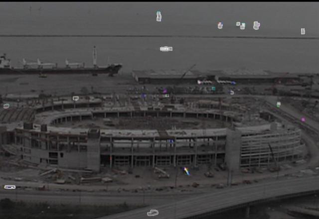
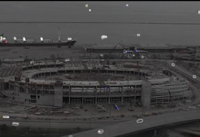
As a bonus, several images were created that highlight the differences between a particular image and the clean image. In each of these images, note the automobile traffic on the local and highway roads, movement in the construction area, and the sailing ships on the lake. Click on each image for a full sized view.
Written by Bob Clodfelter, last updated 28 May 1998.