Coordinate images have z-values proportional to x and y coordinate
values. Suppose we want to define the domain of the image as a rectangular
area -2.5 <= x <= 2.5 and -2.5 <= y <= 2.5:
x = linspace(-2.5,2.5,256);
y = linspace(2.5,-2.5,256);
x = ones(256,1)*x;
y = y' * ones(1,256);
imshow((x+2.5)/5);
imwrite((x+2.5)/5,'x.jpg');
imshow((y+2.5)/5);
imwrite((y+2.5)/5,'y.jpg');
 |  |
| x.jpg | y.jpg |
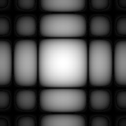
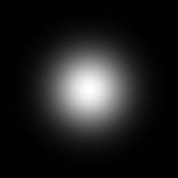
This example generates an image of a two-dimensional gaussian function:
rsq = x.*x + y.*y;
imshow(sqrt(rsq)/5);
imwrite(sqrt(rsq)/5,'r.jpg');
z = exp(-rsq);
imshow(z);
imwrite(z,'gauss.jpg');
z = sinc(x).*sinc(y);
z = z.^2;
imshow(z);
imwrite(z,'sincxy.jpg');
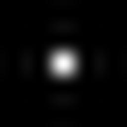
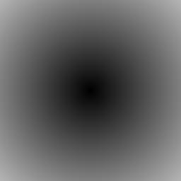
The sinc function has a ring structure which can be seen more clearly
by taking the logarithm of the image. The method is
v = 1.0+log10(v)/decades
where v is a pixel value and decades
is the number of decades to stretch.
decades = 4.0;
v = z;
t = 10^-decades;
v = z.*(z>=t) + (z<t)*t;
v = 1 + log10(v)/decades;
imshow(v);
imwrite(v,'log_sincxy.jpg');
Maintained by John Loomis, last updated 22 May 1998