Finding differences in images

Original images

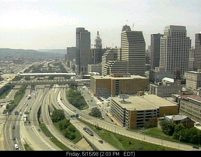
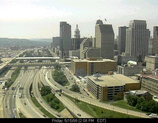
These are jpeg compressed images of downtown Cincinnati.

>> m1 = imread('lytle007.jpg');
>> imshow(m1);
>> m2 = imread('lytle008.jpg');
>> imshow(m2)
>> whos
  Name      Size         Bytes  Class

  m1      501x642x3     964926  uint8 array
  m2      501x642x3     964926  uint8 array

Grayscale conversion

>> d1 = rgb2gray(m1);
>> d2 = rgb2gray(m2);
>> whos
  Name      Size         Bytes  Class

  d1      501x642       321642  uint8 array
  d2      501x642       321642  uint8 array
  m1      501x642x3     964926  uint8 array
  m2      501x642x3     964926  uint8 array

Converting image (uint8) to Double

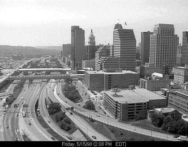
We must convert the uint8 (byte) arrays to double before taking differences because unsigned integers can not represent negative differences. Note that uint8 values range from 0-255, but double image values are expected to range from 0-1.

>> d1 = im2double(d1);
>> d2 = im2double(d2);
>> imwrite(d2,'d2.jpg');

im2double is available in version 2.1 of the image processing toolbox. In our example, the function is equivalent to

>>  d1 = double(d1)/255;

Image Difference

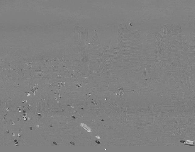
>> diff = d2 - d1;

 max(max(diff)) =  0.9961
 min(min(diff)) = -0.9333

One way of illustrating differences is to map the image range -1 .. 1 into 0 .. 1 by

>> cdiff = (diff+1.0)/2.0;
>> imwrite(cdiff,'cdiff.jpg');

Difference Histogram

>> imhist(cdiff);

Matlab figures can be captured to image files by using the function saveplot defined below:

function SAVEPLOT(name)
%
%SAVEPLOT
%
% Captures active figure and saves it as specified name

[fig,map] = capture;
imwrite(fig,map,name);

The spread in differences could be caused by changes in lighting or camera (recording) parameters. It may also be an effect of image compression.

Here is another way of showing the histogram:

>> [counts,x] = imhist(cdiff);
>> stem(counts,x)
>> stem(x,counts)
>> saveplot stem.tif

Locating Extreme Differences

The extreme differences in these example images are due mostly to traffic. We can see these differences in the "difference" image, but they may be difficult to correlate with static (common) features. The following operations produce a color-coded grayscale image that highlights regions of extreme differences.

» k1 = diff <-0.15; » k2="diff">  0.15;
» g = (d1.*not(k1)).*not(k2);
» final = cat(3,g+double(k2),g,g+double(k1));
» imwrite(final,'final.jpg');

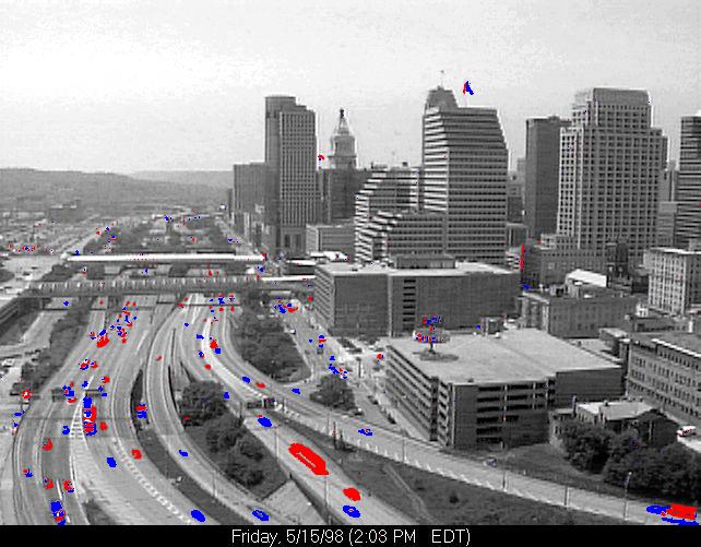
The final image highlights the traffic. There are also a couple of waving flags.

Maintained by John Loomis, last updated 22 May 1998