Cross Correlation

The complex cross correlation of f(x) with g(x) is defined as

The definition can also be written as

after changing the dummy variable of integration. The corresponding definition of cross correlation for sequences would be

Some authors define cross correlation as

The corresponding definition for sequences would be

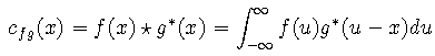
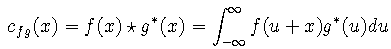
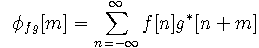
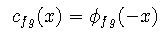
The Matlab function xcorr uses the second definition. Note that

Example 1

Use the following real input sequences:

x = [1 2 3 4];
y = [-1 2 1 -1];

Matlab convolution:

conv(x,y)

ans =

    -1     0     2     3     9     1    -4

The following should be the first definition of cross-correlation:

conv(x,fliplr(y))

ans =

    -1    -1     1     2     8     5    -4

This should be the second definition of cross-correlation:

conv(fliplr(x),y)

ans =

    -4     5     8     2     1    -1    -1

and indeed it does match the results of xcorr:

xcorr(x,y)

ans =

   -4.0000    5.0000    8.0000    2.0000    1.0000   -1.0000   -1.0000

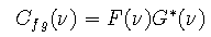
Fourier Transform of Cross-Correlation Function

Using the first definition of cross correlation, we can find its Fourier transform as

Example 2

To insure linear convolution (rather than cyclic convolution) we must zero pad the input sequences:

x = [ 1 2 3 4 0 0 0 0];
y = [ -1 2 1 -1 0 0 0 0];

Now we generate the cross correlation (first definition) and check that it is a real sequence so that we can eliminate the spurious small imaginary component due to round-off

xc = ifft(fft(x).*conj(fft(y)));
max(abs(imag(xc)))

ans =
   1.0413e-15

xc = real(xc)

We use fftshift to display the results in the correct order

t = [ 0 1 2 3 -4 -3 -2 -1];
[fftshift(t)' fftshift(xc)']

ans =
   -4.0000    0.0000
   -3.0000   -1.0000
   -2.0000   -1.0000
   -1.0000    1.0000
         0    2.0000
    1.0000    8.0000
    2.0000    5.0000
    3.0000   -4.0000

Finally we compare to the results of xcorr

[xco,lags] = xcorr(x,y);
[lags' xco']

ans =

   -7.0000    0.0000
   -6.0000    0.0000
   -5.0000   -0.0000
   -4.0000   -0.0000
   -3.0000   -4.0000
   -2.0000    5.0000
   -1.0000    8.0000
         0    2.0000
    1.0000    1.0000
    2.0000   -1.0000
    3.0000   -1.0000
    4.0000   -0.0000
    5.0000         0
    6.0000    0.0000
    7.0000    0.0000

The results are the same if we change the sign of the lags.

Example 3

Consider the following complex sequences:

x = [ 1+3j 2 3-j 4+j]
x =
   1.0000 + 3.0000i   2.0000             3.0000 - 1.0000i   4.0000 + 1.0000i

y = [ -1+j 2-j 1 -1-j]
y =
  -1.0000 + 1.0000i   2.0000 - 1.0000i   1.0000            -1.0000 - 1.0000i

We append zeros, as before, to insure linear convolution when using the finite discrete fourier transform:

xz = [x zeros(1,4)];
yz = [y zeros(1,4)];

First we demonstrate the use of the Matlab function xcorr:

[xco, lags] = xcorr(x,y);
[lags' xco']

ans =

  -3.0000            -3.0000 + 5.0000i
  -2.0000             3.0000 - 4.0000i
  -1.0000             9.0000 - 0.0000i
        0             4.0000 - 0.0000i
   1.0000            -1.0000 -11.0000i
   2.0000            -1.0000 - 5.0000i
   3.0000            -4.0000 + 2.0000i

Next we demonstrate the use of the Fourier transform (based on first definition of cross correlation):

xc = ifft(fft(xz).*conj(fft(yz)));
t = [0 1 2 3 -4 -3 -2 -1];
[fftshift(t)' fftshift(xc)']

ans =

  -4.0000                  0 + 0.0000i
  -3.0000            -4.0000 + 2.0000i
  -2.0000            -1.0000 - 5.0000i
  -1.0000            -1.0000 -11.0000i
        0             4.0000 - 0.0000i
   1.0000             9.0000 - 0.0000i
   2.0000             3.0000 - 4.0000i
   3.0000            -3.0000 + 5.0000i

The results are the same if you change the sign of the lags in xcorr.

We also demonstrate the results obtained from direct convolution:

xcn = conv(x,fliplr(conj(y)));
xcn'

ans =

  -4.0000 + 2.0000i
  -1.0000 - 5.0000i
  -1.0000 -11.0000i
   4.0000          
   9.0000          
   3.0000 - 4.0000i
  -3.0000 + 5.0000i

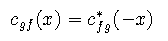
Commutative Property of Cross Correlation

Cross correlation is non-commutative:

using either definition of cross correlation

Example 4

Using the sequences from example 3, we have

xco = xcorr(x,y);
xco'

ans =

  -3.0000 + 5.0000i
   3.0000 - 4.0000i
   9.0000 - 0.0000i
   4.0000 - 0.0000i
  -1.0000 -11.0000i
  -1.0000 - 5.0000i
  -4.0000 + 2.0000i

xrev = xcorr(y,x);
xrev'                                                                                                                            

ans =

  -4.0000 - 2.0000i
  -1.0000 + 5.0000i
  -1.0000 +11.0000i
   4.0000 + 0.0000i
   9.0000 + 0.0000i
   3.0000 + 4.0000i
  -3.0000 - 5.0000i

The second example is the conjugate of the first in reverse order, as expected.

Maintained by John Loomis, last updated 15 Oct 1997