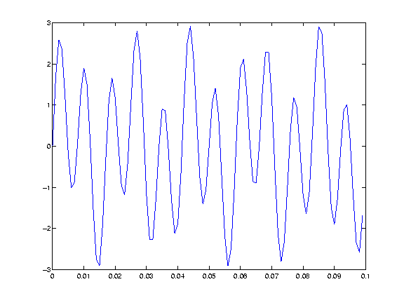
There are a variety of ways of generating waveforms. Most require that you begin with a vector that represents a time base. Consider generating data with a 1000 Hz sample frequency, for example.
>> t = (0:1000)/1000;
>> whos
  Name      Size         Bytes  Class
  t         1x1001        8008  double array
The colon operator creates a 1001-element row vector that represents time from zero to
one second in steps of one millisecond. The command whos displays the name and
size of each current variable.
>> t = t';
>> whos
  Name      Size         Bytes  Class
  t      1001x1           8008  double array
The transpose operator (') changes the row vector to a column vector. The semicolon tells Matlab to compute but not to display the result.
Given t you can create a sample signal y consisting of two
sinusoids, one at 50 Hz and one at 120 Hz with twice the amplitude.
>> y = sin(2*pi*50*t) + 2*sin(2*pi*120*t);
>> plot(t(1:100),y(1:100))
The print command is used to obtain a hardcopy of a plot or to save the
plot as a bitmap file. The command below saves the plot as a Windows 256-color bitmap.
>> print -dbmp256 plot1.bmp
Compare the output above to the results obtained by capturing the contents of the plot window and writing it to a bitmap file.
>> [fig,map]=capture(1);
>> imwrite(fig,map,'plot1.tif');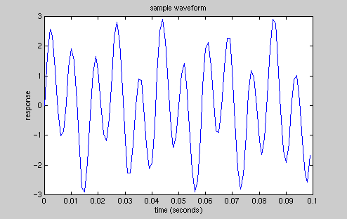
The labels are the result of labeling commands (see below). The colors are those of the
actual window. Note that the print command resulted in a white background.
The size of the bitmap is the same as the size of the graphics window. Try resizing the window and capturing the result to another file.
>> % resize figure window manually
>> [fig2,map] = capture(1);
>> whos
  Name       Size         Bytes  Class
  fig      419x559      1873768  double array
  fig2     232x390       723840  double array
  map       68x3           1632  double array
  t       1001x1           8008  double array
  y       1001x1           8008  double array
There are a variety of commands useful in labeling plots. Here are some examples:
>> xlabel('time (seconds)');
>> ylabel('response');
>> title('sample waveform');
>> [fig3,map] = capture(1);
>> imwrite(fig3,map,'plot1.tif');
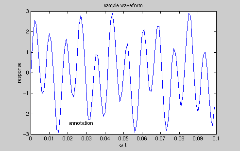
Greek letters and mathematical symbols can be included using TeX notation.
>> xlabel('\omega t')
>> gtext('annotation')
>> [fig4,map] = capture(1);
>> imwrite(fig4,map,'fig4.tif');
>> imwrite(fig4,map,'fig4.bmp');
Utility packages such as lviewpro can designate a color
in a 1989-format gif file as transparent. Most web browsers will display
transparent gif files correctly.

Matlab represents ordinary one-dimensional sampled data signals, or sequences, as vectors. Vectors are 1-by-n or n-by-1 arrays, where n is the number of samples in the sequence.
Column orientation is preferable for single channel signals because it extends naturally to the multichannel case. For multichannel data, each column of the matrix represents one channel. Each row of such a matrix then corresponds to a sample point.
Suppose you define a five-element column vector as follows:
>> a = [1 2 3 4 5];
>> a = a';
To duplicate column vector a into a matrix, use the following method:
>> c = a(:,ones(1,3))

c =

     1     1     1
     2     2     2
     3     3     3
     4     4     4
     5     5     5
A similar method can be used to duplicate a row vector:
>> a = a'

a =

     1     2     3     4     5

>> c = a(ones(3,1),:)

c =

     1     2     3     4     5
     1     2     3     4     5
     1     2     3     4     5
Matlab can import data from outside in several ways.
>> load mtlb
>> specgram(mtlb,512,Fs,kaiser(500,5),475)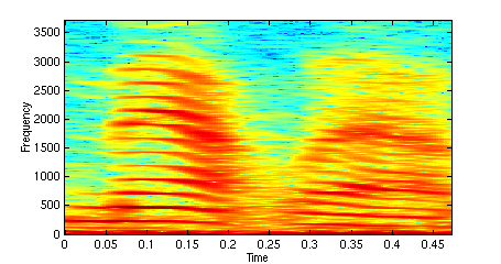
This is a digitized speech signal. You may play it using the command
>> sound(mtlb,Fs)
The program datagen.cpp (download datagen.zip creates a file called sample.dat. The data for a exponentialed damped sine and cosine are calculated and saved in three columns of numbers.
On the SUN, you would use the following commands to compile and run this program
CC -o datagen datagen.cpp
datagen
To read and plot the data, you may use the following
>> load sample.dat
>> whos sample
  Name         Size         Bytes  Class
  sample     501x3          12024  double array

>> x = sample(:,1);
>> y = sample(:,2);
>> z = sample(:,3);
>> plot(x,y)
>> hold
Current plot held
>> plot(x,z)
>> hold off

>> [fig2,map] = capture(1);
>> imwrite(fig2,map,'fig2.tif');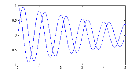
The
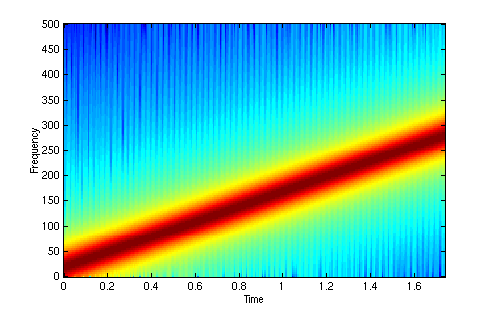
To compute 2 seconds of a linear chirp signal with a sample rate of 1 kHz, that starts at
DC and crosses 150 Hz at 1 second, use
To plot the spectrogram use
To change the colormap to gray-levels use
The function
The
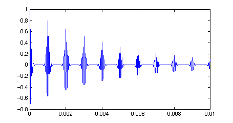
The following example generates a pulse train consisting of the sum of multiple
delayed interpolations of a Gaussian pulse. The pulse train is defined to have a sample rate
of 50 kHz, a length of 10 msec, and a pulse repetition rate of 1KHz. The array d specifies
the delay to each pulse repetition in column 1 and an optimal attenuation for each repetition in
column 2.
The pulse train is constructed by passing the name of the The function
chirp
function generates a linear swept-frequency cosine signal. An optional parameter
specifies alternative sweep methods. An optional parameter phi allows the initial
phase to be specified in degrees.
>> t= (0:2000)/1000;
>> y = chirp(t,0,1,150);
>> specgram(y,256,1000,256,250);
>> [fig5,map]=capture(1);
>> imwrite(fig5,map,'fig5.tif');
>> colormap(gray(250));
>> [fig5g,map]=capture(1);
>> imwrite(fig5g,map,'fig5g.tif');

Dirichlet Function
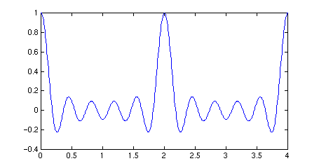
diric computes
the Dirichlet function, sometimes called
the periodic sinc or aliased sinc function.
>> t = linspace(0,4,500);
>> yd = diric(pi*t,11);
>> plot(t,yd)
Pulstran Function
pulstran
function generates pulse trains from either continuous or sampled prototype pulses.
gauspuls function to
pulstran, along with additional parameters that specify a 10 kHz Gaussian pulse
with 50% bandwidth.
>> Fs = 50e3; % 50kHz
>> length = 10e-3; % 10 msec
>> t = 0:1/Fs:length;
>> d = [(0:10)/1E3; 0.8.^(0:10)]';
>> yf = pulstran(t,d,'gauspuls',10E3,0.5);
>> plot(t,yf);
Sinc Function
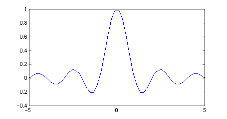
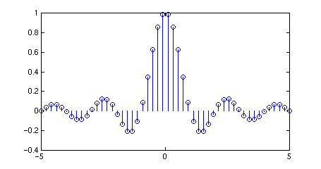
sinc
computes the mathematical sinc function, sinc(x) = sin(pi*x)/(pi*x).
t = linspace(-5,5,50);
yc = sinc(t);
plot(t,yc);
[fig6,map] = capture(1);
imwrite(fig6,map,'fig6.tif');
 stem(t,yc);
[fig6s,map] = capture(1);
imwrite(fig6s,map,'fig6s.tif');
Maintained by John Loomis, last updated Aug 7, 1997