Sinc Interpolation Examples

Matlab code for sinc interpolation

function y = sinc_interp(x,u)

m = 0:length(x)-1;

for i=1:length(u)
  y(i) = sum(x.*sinc(m- u(i)));
end

Example 1

The function is the sequence x[n] = n a^n u[n].

a = 0.9;
N = 64;
n = 0:N-1;
x = n.*a.^n;

Sampled values

plot(n,x);

Magnitude of Fourier transform

The function is essentially band-limited

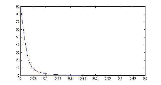
y = fft(x);
k= 0:N/2;
plot(k/N,abs(y(1:N/2+1)));

Interpolations

The black curve is the Matlab interp method. The blue curve is sinc interpolation. The circles are sample values.

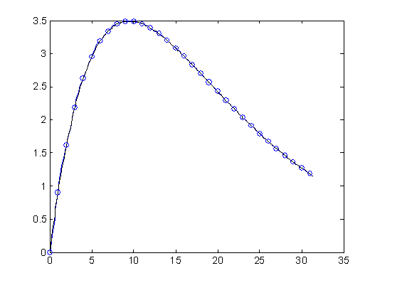
s = linspace(0,63,512);
x2 = sinc_interp(x,s);
plot(s(1:256),x2(1:256));
hold
xi = interp1(n,x,s);
plot(s(1:256),xi(1:256),'k');
plot(n(1:N/2),x(1:N/2),'o');
hold off

The first half of the data is shown.

Interpolation difference

The following shows the difference between the two interpolation methods.

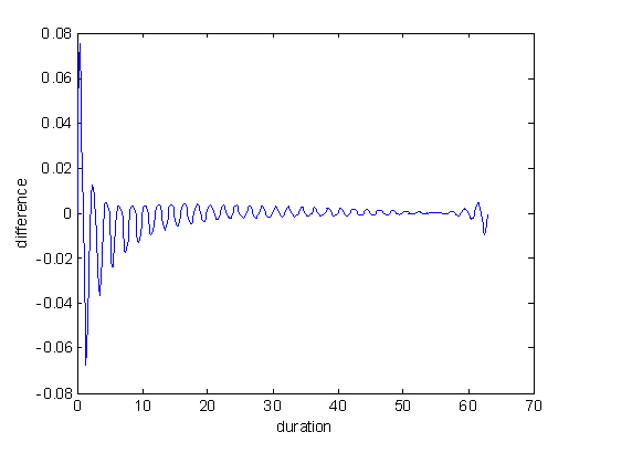
plot(s,xi-x2);
ylabel('difference');
xlabel('duration');

Example 2

The function is the sequence x[n] = a^n u[n].

a = 0.9;
N = 64;
n = 0:N-1;
x = a.^n;

Sampled values

Magnitude of Fourier transform

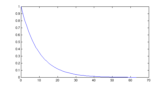
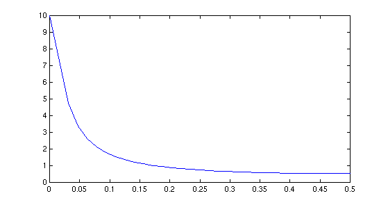
Not exactly band-limited

Interpolations

The black curve is the Matlab interp method. The blue curve is sinc interpolation. The circles are sample values.

Interpolation difference

Conclusion

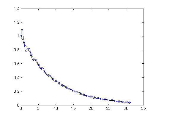
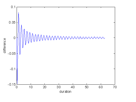
sinc interpolation is seldom optimal. It almost always exhibits ringing, sometimes severely.

Maintained by John Loomis, last updated 26 Oct 2005