 |  |
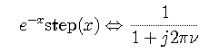
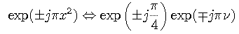
There are a number of special functions used in studying signal processing either because they can be used to model typical physical systems or because they are the result of Fourier transforming simple functions.
| |
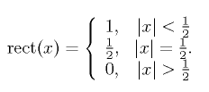
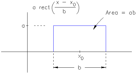
The equation on the left is the basic definition of the rectangle function. The chart on the right shows a rectangle function of height a and width b, centered at the location x_0.
 |  |
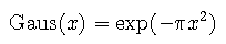 | 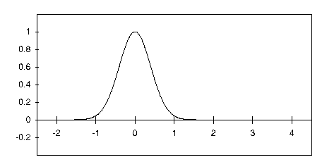 |
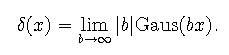
The Gaussian function Gaus(x) is defined with a factor of pi in the exponent. When defined in this fashion, the Gaussian function has a height and area of unity.
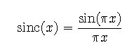 | 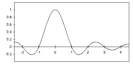 |
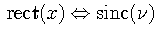
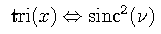
The sinc function sinc(x) contains an explicit factor of pi in its definition. This definition gives the sinc function a height and area of unity and integral values for the zeros of the function. The sinc function is the Fourier transform of the rectangle function.
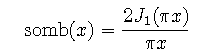 |  |
The sombrero function somb(x) is the two-dimensional polar-coordinate analog of the sinc function. It is defined using the first-order Bessel function of the first kind in place of the sine function. The sombrero function somb(r) has a central ordinate of unity and a volume of 4/pi.
 | 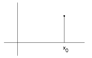 |
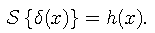
The impulse function, also known as Dirac's delta function, is used to represent quantities that are highly localized in space. Examples include point optical sources, electrical charges, or masses.
The impulse function can be visualized in a number of ways. One way
is to think of it as a narrow spike having infinite height
and zero width such that its area is equal to unity. Another way is
to think of the impulse function  as the result of a
limiting process obtained by taking a sequence of functions, such
as the Gaussian function, with unit area but variable height and
width, and then defining the impulse function as
as the result of a
limiting process obtained by taking a sequence of functions, such
as the Gaussian function, with unit area but variable height and
width, and then defining the impulse function as
As b increases the members of the sequence become narrower and taller, as shown in the figure above, but their area remains constant. A final way of thinking about the impulse function is to consider it as so localized that its actual shape is no longer observable and any further decrease in size would not affect the results of the problem under consideration.
The impulse function may also be defined from its basic properties. Given a complex-valued function f(x),
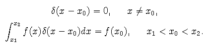
If f(x) is discontinuous at the point x=x_0, the value of f(x_0) is taken as the average of the limiting values as x approaches x_0 from above and below. On graphs we will represent the delta function as a spike of unit height as shown above, but we must remember that the height of the spike represents the area of the impulse function.
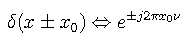
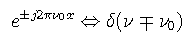
The impulse function often appears with a scaled argument. The following scaling rule applies,
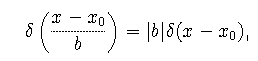
which may be derived from the defining properties. A simple application of the scaling rule gives
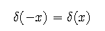
which shows that the impulse function is an even function.
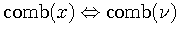
The comb function is an array of delta functions
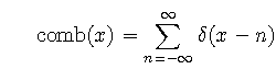
where n takes on integer values. The translated and scaled version of the comb function is
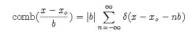
A comb function is used to sample another continuous function f(x) at equal intervals.
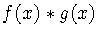
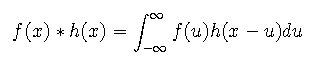
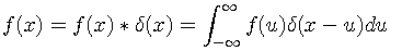
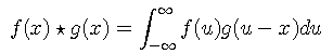
The convolution of two functions f(x) and h(x) in one dimension is denoted as f(x) * g(x) and defined by the following integral.
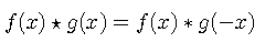
Convolutions are associative, distributative, and commutative. These same properties are shared with the operations of multiplication and integration, from which convolution is defined.
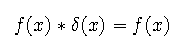
Convolution of the impulse function with any other function f(x) reproduces the other function.
If either function in a convolution is shifted by an amount x_0, the resulting convolution is shifted by the same amount.

where g(x) = f(x) * h(x).
where g(x) = f(x) * h(x).
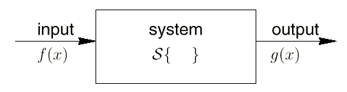
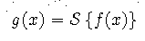
The modeling of physical systems is often represented by mathematical operators. In the figure above the input image or signal f(x) is transformed by the operator S into the output image or signal g(x). This process can be represented by the expression,
A linear system is one that obeys the principle of superpostion,
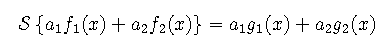
where the output of a linear combination of inputs is the same linear combination applied to the individual outputs. This result means that a complicated system can be decomposed into a linear combination of elementary functions whose transformation is known, and then taking the same linear combination of the results. Linearity also implies that the behavior of the system is independent of the magnitude of the input.
A system is said to be shift invariant if the only effect caused by a shift in the position of the input is an equal shift in the position of the output, that is
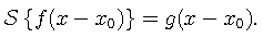
The magnitude and shape of the output are unchanged, only the location of the output is changed.
When the input to a system is a single impulse, the output is called the impulse response. Let h(x) be the impulse response, given by
A general function f(x) can be represented as a linear combination of impulses, since
Then, using the principle of superposition,
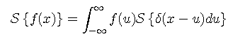
and finally after incorporating the impulse response,
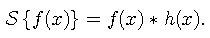
This very important result says that the output of any linear, shift-invariant system is given by the convolution of the input with the impulse response of the system.
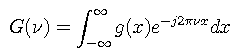
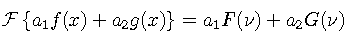
To represent a nonperiodic function g(t) everywhere, an integral expansion known as the Fourier transform is required.
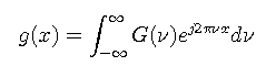
where
The function f(x) which is periodic with period
 can be represented everywhere by a Fourier series
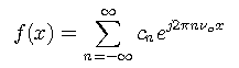
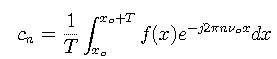
where
Given
 | and | 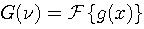 |
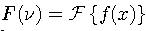
The transform of a sum of two functions is the sum of their individual transforms.
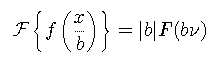
If the width of a function is increased, keeping the height constant, its Fourier transform becomes narrower and taller.
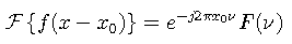
The Fourier transform of a translated function is the transform of the untranslated function multiplied by a linear phase factor.
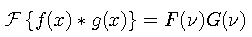
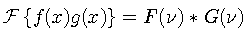
The Fourier transform of a product of two functions is the convolution of the individual transforms.
 |  |
| Real, even | Real, even |
| Real, odd | Imaginary, odd |
| Real, no symmetry | Hermetian: Even real part, odd imaginary part |
| Imaginary, even | Imaginary, even |
| Imaginary, odd | Real, odd |
| Imaginary, no symmetry | Antihermetian: Odd real part, even imaginary part |
| Complex, even | Complex, even |
| Complex, odd | Complex, odd |
| Complex, no symmetry | Complex, no symmetry |
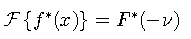
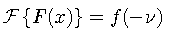
This property allows us to use Fourier pairs in reverse

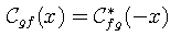
This definition differs from a convolution in that the shifted function is not inverted. One of the major consequences of this difference is that the cross-correlation operation (unlike convolution) is not commutative. Cross-correlation can be expressed as the following convolution,
For complex functions, we define cross-correlation as
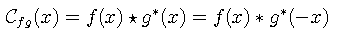
and can show that
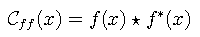
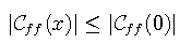
The complex autocorrelation function is hermitian, that is its real part is even and its imaginary part is odd. It also has the important property that its modulus is maximum at the origin, namely
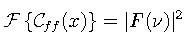
The Fourier transform of the complex autocorrelation function is given by
Maintained by John Loomis, last updated 5 Sept 1997