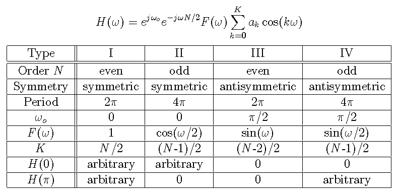


b = [ 1 0 1 ]/2;
plotfir(b);
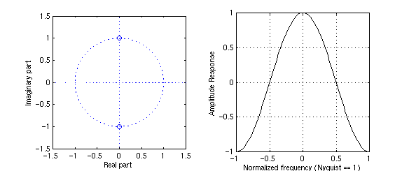
b = [ 1  1 ]/2;
plotfir(b);
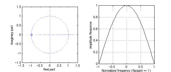
b = [ 1 0 -1 ]/2;
plotfir(b);
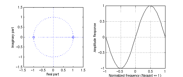
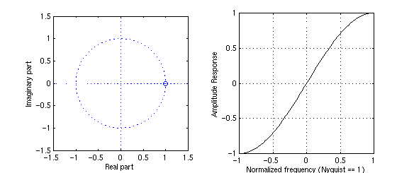
b = [ 1 -1 ]/2;
plotfir(b);
All of these filters are generated by b = ones(1,M)/M.
b = ones(1,2)/2;
plotfir(b);

b = ones(1,3)/3;
plotfir(b);
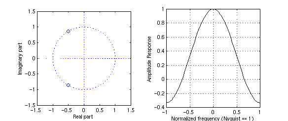
b = ones(1,4)/4;
plotfir(b);
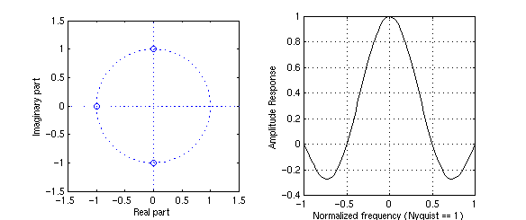
b = ones(1,5)/5;
plotfir(b);
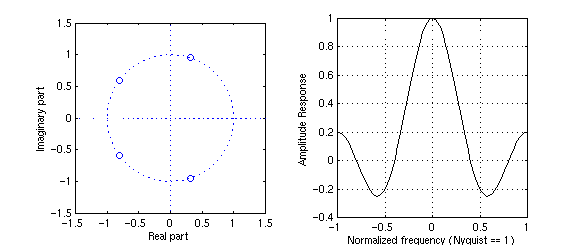
This filters are obtained by repeated convolution of a M = 2 moving average filter.
b2 = ones(1,2)/2;
b3 = conv(b2,b2);
b4 = conv(b2,b3);
b5 = conv(b2,b4);
b2 = [1 1]/2;

b = [ 1 2 1]/4;

b = [ 1 3 3 1]/8;
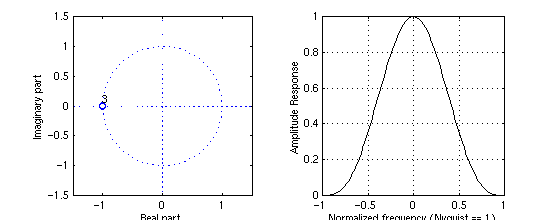
b = [ 1 4 6 4 1]/16;

plotfir functionfunction PLOTFIR(b) % % PLOTFIR % % generates set of plots for rational transfer function % defined by a set of zeros and poles. % % PLOTFIR(b) N = length(b)-1; a = [ 1 zeros(1,N) ]; [h,w] = freqz(b,a,2*pi*linspace(-0.5,0.5,100)); h = h.*exp(j*w*N/2); if (max(abs(imag(h))) > 0.5) h = -j*h; end h = real(h); subplot(1,2,2); plot(w/pi,h,'k'); grid xlabel 'Normalized frequency (Nyquist == 1)' ylabel 'Amplitude Response' subplot(1,2,1); [z,p,k] = tf2zp(b,a); zplane(z,[]); axis([-1.5 1.5 -1.5 1.5]);
Maintained by John Loomis, last updated 30 Oct 1997