A very general class of linear shift-invariant systems can be constructed from a linear, constant-coefficient difference equation of the form

The following MATLAB functions are discussed:
filterThe MATLAB filter implements this class of systems.
y = filter(b,a,x) filters the data in vector x with the filter
described by coefficient vectors a and b to create the filtered
data vector y.
When x is a matrix, filter operates on the columns of x.
When x is an N-dimensional array, filter operates on the
first non-singleton dimension. filter works for both real and complex inputs.
The filter coefficients in MATLAB start with the subscript 1, rather than 0.
If a(1)  1,
1, filter normalizes the filter coefficients by a(1). If
a(1) = 0, the input is in error.
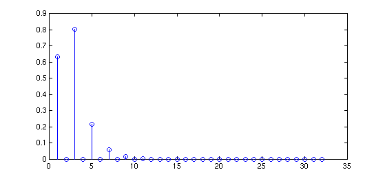
Consider the filter y[n] - 0.268 y[n-2] = 0.634 x[n] + 0.634 x[n-2]. Generate the impulse response.
>> a = [1 0 -0.268]

a =

    1.0000         0   -0.2680

>> b = [0.634 0 0.634]

b =

    0.6340         0    0.6340

>> x = [1 zeros(1,31)];
>> y = filter(b,a,x);
>> y = stem(y);
>> [fig,map] = capture(1);
>> imwrite(fig,map,'filter_example.tif');

filter is a built-in MATLAB function. filter
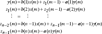
is implemented as a transposed direct form II structure

where n-1 is the filter order.
The operation of filter at sample m
is given by the time domain difference equations for y and the states
zi :

You can use filtic to generate the state
vector zi(0) from past inputs and outputs.
The input-output description of this filtering operation in the z-transform domain is a rational transfer function:

impz[h,t] = impz(b,a) computes
the impulse response of the filter with numerator coefficients b
and denominator coefficients a. impz chooses the number
of samples and returns the response in column vector h and times
(or sample intervals) in column vector t (where t = (0:n-1)'
and n is the computed impulse response length).
[h,t] = impz(b,a,n) computes
n samples of the impulse response. If n is a vector of integers, impz computes
the impulse response at those integer locations where 0 is the starting
point of the filter.
[h,t] = impz(b,a,n,Fs) computes
n samples and scales t so that samples are spaced 1/Fs
units apart. Fs is 1 by default.
[h,t] = impz(b,a,[],Fs) chooses
the number of samples for you and scales t so that samples are
spaced 1/Fs units apart.
impz with no output
arguments plots the impulse response in the current figure window using
stem(t,h).
impz works for both real and complex input systems.
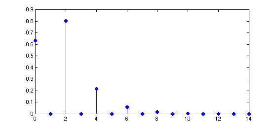
The impulse response for the previous example could have been generated with a
single call to impz.
>> impz(b,a)
>> [fig,map] = capture;
>> imwrite(fig,map,'impz.tif');

impz filters a length n impulse
sequence using
filter(b,a,[1 zeros(1,n-1)])
To compute n in the auto-length case, impz
either uses n = length(b) for the FIR case or first finds the
poles using p = roots(a), if length(a) is greater than 1.
If the filter is unstable, n is chosen
to be the point at which the term from the largest pole reaches 10^6
times its original value.
If the filter is stable, n is chosen to
be the point at which the term due to the largest amplitude pole is 5*10^-5
of its original amplitude.
If the filter is oscillatory (poles on the unit
circle only), impz computes five periods of the slowest oscillation.
If the filter has both oscillatory and damped terms,
n is chosen to equal five periods of the slowest oscillation or
the point at which the term due to the largest (nonunity) amplitude pole
is 5*10^-5 of its original amplitude, whichever is greater.
impz also allows for delay in the numerator
polynomial, which it adds to the resulting n.
freqzfreqz returns the complex frequency response
H(ejw) of a digital filter, given the numerator
and denominator coefficients in vectors b and a.
[h,w] = freqz(b,a,n) returns the n-point
complex frequency response of the digital filter

given the coefficient vectors b and a.
freqz returns both h, the complex frequency response,
and w, a vector containing the n frequency points. freqz
evaluates the frequency response at n points equally spaced around
the upper half of the unit circle, so w contains n points
between 0 and  .
.
It is best, although not necessary, to choose a value
for n that is an exact power of two, because this allows fast
computation using an FFT algorithm. If you do not specify a value for n,
it defaults to 512.
[h,f] = freqz(b,a,n,Fs) specifies
a positive sampling frequency Fs, in Hertz. It returns a vector
f containing the actual frequency points between 0 and Fs/2
at which it calculated the frequency response. f is of length
n.
[h,w] = freqz(b,a,n,'whole') and
[h,f] = freqz(b,a,n,'whole',Fs) use
n points around the whole unit circle (from 0 to 2 , or from 0 to
 Fs).
h = freqz(b,a,w) returns
the frequency response at the frequencies in vector w. These frequencies
must be between 0 and 2 .
.
h = freqz(b,a,f,Fs) returns
the frequency response at the frequencies in vector f, where
the elements of f are between 0 and Fs.
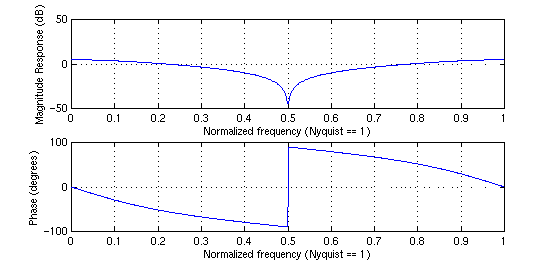
freqz with no output arguments plots the
magnitude and phase response versus frequency in the current figure window.
freqz works for both real and complex input systems.
The frequency response for the example filter can be generated as:
single call to impz.
>> freqz(b,a);

Warning: Log of zero.
> In /usr/local/matlab/toolbox/matlab/elfun/log10.m at line 13
  In /usr/local/matlab/toolbox/signal/freqz.m at line 120
>> [fig,map] = capture;
>> imwrite(fig,map,'freqz.tif');
The warning messages here can be ignored

freqz uses an FFT algorithm when argument
n is present. It computes the frequency response as the ratio
of the transformed numerator and denominator coefficients, padded with
zeros to the desired length:
h = fft(b,n)./fft(a,n)
If n is not a power of two, the FFT algorithm
is not as efficient and may cause long computation times.
When a frequency vector w or f
is present, or if n is less than max(length(b),length(a)),
freqz evaluates the polynomials at each frequency point using
Horner's method of polynomial evaluation and then divides the numerator
response by the denominator response.
Maintained by John Loomis, last updated 11 Sept, 1997