Download lab6 materials
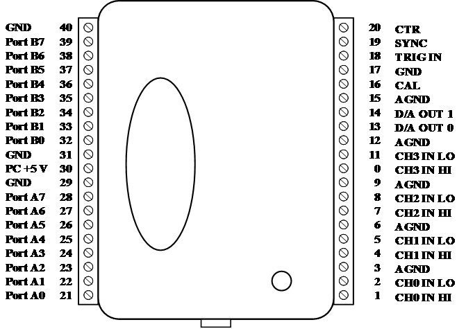
You will be using the USB-1208FS data acquisition system. The USB-1208FS features four 12-bit analog diffential input signal connections, two analog output signal connections, and 16 digital I/O lines. It is powered by the +5 volt USB supply. No external power is required.
You will need to install the daq using InstaCal, which can be obtained from the MCC downloads page.
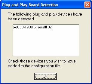
When you run InstaCal, you should get a "PlugandPlay" window like the one below
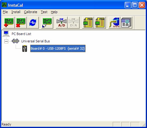
Afterwards the InstaCal screen should look something like the following screenshot.
Perform the following test:
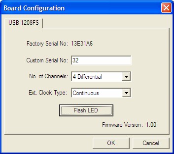
Select menu: Install — Config .... Press "Flash LED" button
MATLAB supports a variety of data acquisition systems in the Data Acquisition Toolbox. To perform any task with your data acquisition application, you must call M-file functions from the MATLAB environment. Among other things, these functions allow you to:
Close InstalCal before starting MATLAB.
Run daq_info.m
script to verify operation of daq in MATLAB.
If you are having trouble running the daq in Vista or Windows 7, see the following link.
As you make electrical measurements, whether by a multimeter or an oscilloscope, you often observe that the least significant digit (or more) fluctuates over time. This is true of samples from an A/D converter, even if the input is a constant DC value. Below is a histogram of values obtained from repeated samples of a constant voltage.
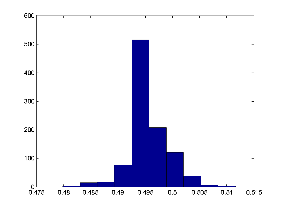
In a complete test, you should plot samples as a function of time and look for any systematic trends. Assuming there are no apparent trends, the remaining fluctuations are considered noise. The width of the distribution (spread of values) measures the amount of noise.
In addition, we note that the values are quantized. There are distinct groups of values. The quantization step is related to the resolution of the A/D converter. If there are N bits, then there are 2N distinct values and 2N-1 distinct steps. The step size is the total range in volts, divided by the number of steps. If you know the step size, you can work backwards to the number of steps and then the number of bits.
The sampling theorem says that if you sample faster than the Nyquist rate (twice the maximum frequency present in the signal) and you sample for a very long time (approaching infinity), then you can reconstruct the original continuous signal by sinc interpolation.
If, as is often the case, you have only a relatively small number of samples, applying sinc interpolation leads to Gibb's phenomenon oscillations. A better interpolation method, suitable for a limited range of samples, is spline interpolation. MATLAB has an interpolation function interp1.m for which spline interpolation is an option.
The diagram below shows a continuous sinusoid (dashed blue plot) whose frequency is close to the Nyquist frequency. The available samples are shown with circular markers. The solid black curve shows the result of using spline interpolation to generate intermediate values.
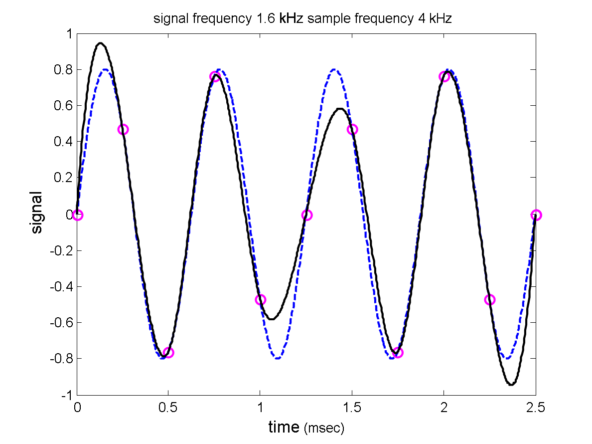
The resulting reconstruction is not bad, but it is distinctly not sinusoidal. Here is the MATLAB script for this calculation.
Maintained by John Loomis, last updated 10 Nov 2010