
Summary
Virtual reality is hot, and as the number-crunching power of today's computers increases, it's certain to become even hotter. Wouldn't it be really cool to build your own virtual reality? It's not so far fetched; you can do it -- if you have the right tools and the know-how. And that's what I'm here for. This column kicks off a series on three-dimensional computer graphics. Over the next three months, I'm going to teach you the techniques and demonstrate them in action. You'll learn how to build a three-dimensional model, and how to view the model on a computer screen. You'll also learn how to handle perspective, shading, rotation, and translation. By the time you finish, you'll know enough to create your own virtual reality.So listen up; you don't want to be left behind. (2,200 words)
![]()
Explore your world
As far as I know, we can't just stick a bit of our world directly
inside a computer (without damaging the computer, anyway). The best we
can do is to create a computer model of our world. Given that limitation,
how do we model something like a chair, for example?
Objects in our world have characteristics, or properties, such as shape, size, weight, position, orientation, and color (and the list goes on and on). Let's consider for a moment only their shape, position, and orientation -- these properties are what we call spatial properties. And let's start with something easier to work with than a chair -- a cube, for example.
Take a look at the illustration in Figure 1. It shows a cube sitting in an otherwise empty room. (Well okay, the room has a door, too, but that's there only to make the room look more like a room.)
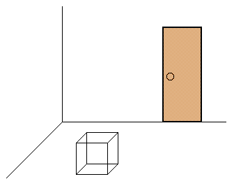
Figure 1: A room with a cube
In order to specify the shape, position, and orientation of a cube we need to specify the location of each of its corners. In order to do that, we could use language like this:
The first corner is a foot (or meter, if you prefer) above the floor and two and a half feet (or meters) from the wall behind me. The second corner is also a foot above the floor and a foot from the wall to my left....
Note that both of the corners were specified relative to something else (the wall and/or the floor). In our computer model, we could define a floor and a wall and use them as points of reference, but it turns out to be much easier to simply select one point of reference (which we'll call the origin) and use that instead. For our origin, we'll use the corner formed by the two walls and the floor. Figure 2 indicates the location of our origin.
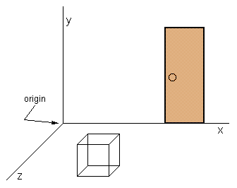
Figure 2: The origin and the coordinate axis
Now we need to indicate where each corner is located with respect to the origin. You can specify the path from the origin to a corner of the cube in a number of ways. For simplicity, we must agree on a standard. Let's do the following:
Imagine that each of the edges formed by the intersection of a wall and a wall, or a wall and the floor, is given a name -- we'll call them the x axis, the y axis, and the z axis, as indicated in Figure 2. And let's also agree up front that we'll determine the location of a corner by following this recipe:
Figure 3 shows the path we would follow to get to one of the cube's corners.
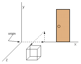
Figure 3: Finding your path
As a shorthand notation, let's write all of these distances as:
or (even shorter):
(distance x,distance y,distance z)
This triplet of values is called the corner's coordinates. We can specify the position in space of each corner in a similar manner. We might find, for example, that the cube is this example has corners at:
(3 feet, 1 foot, 2 feet)
or
(3 feet, 1 foot, 3 feet)
or
(4 feet, 1 foot, 2 feet)
and so on.
The units of measurement (feet, meters, for example) aren't important for our purposes. What is important is how the units map to the standard unit of screen real estate -- the pixel. I'll talk more about that mapping a bit later.
Getting a little edgy
The location of the cube's corners determines the position and
orientation of the cube. However, given only the coordinates of
its corners, we can't reconstruct a cube (much less a chair). We really
need to know where the edges are, because the edges determine shape.
All edges have one very nice characteristic -- they always begin and end at corners. So, if we know where all the edges are, we will certainly know where all the corners are.
Now we're going to make one big simplifying assumption. In our model of the world, we are going to outlaw curved edges (you'll learn why later); edges must always be straight lines. To approximate curved edges, we'll lay straight edges end-to-end, as in Figure 4.
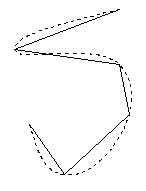
Figure 4: The straight line approximation of a curve
Edges then become nothing more than simple line segments. And line segments are specified by the coordinates of their begin and end points. Therefore, the model of an object is nothing more than a collection of line segments that describe its shape.
Visualization: It's not just for relaxation anymore
Now that we know how to model an object, we are ready to tackle
the problem of representing a model on the computer screen.
Think of the computer screen as a window into our virtual world. We sit on one side of the window, and the virtual world sits on the other. Figure 5 illustrates this concept.
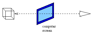
Figure 5: Our window into the virtual world
There are many ways to put the information in the model on the window (or computer screen). Possibly the simplest is what is called an isometric projection.
Because our model has three dimensions and the computer screen has only two, we can map the model to the screen by first removing the z coordinate (the third of the three coordinates) from each point in the model. This leaves us with the x and y coordinates for each point. The x and y coordinates are scaled appropriately (based on the units of the model) and mapped to the pixels on the screen. We can use these steps on any point of interest in the model to find out where it would appear on the screen.
As it turns out, it's not necessary to transform every point in our model this way. One of the consequences of having approximated every edge in the model with line segments is that we really need only transform the end points of a line segment, not every point on the line segment. This is true because simple projections (like an isometric projection) always transform line segments into line segments -- line segments don't become curves. Therefore, once you know the positions of the transformed end points, we can use the AWT's built-in line drawing routines to draw the line segment itself.
I think an example might be in order. I'm going to create three simple models of the same shape in different orientations.
Table 1 contains the data describing a simple shape in its first position. Each row in the table corresponds to an edge. The table gives the coordinates of the edge's begin and end points. Let's assume we're looking at the shape from out along the z axis.
| Segment | Begin | End | ||||
|---|---|---|---|---|---|---|
| x | y | z | x | y | z | |
| A | 25 | 0 | -70 | 25 | 35 | -35 |
| B | 25 | 35 | -35 | 25 | 0 | 0 |
| C | 25 | 0 | 0 | 25 | -35 | -35 |
| D | 25 | -35 | -35 | 25 | 0 | -70 |
| E | 25 | 0 | -70 | -25 | 0 | -70 |
| F | -25 | 0 | -70 | -25 | 35 | -35 |
| G | -25 | 35 | -35 | -25 | 0 | 0 |
| H | -25 | 0 | 0 | -25 | -35 | -35 |
| I | -25 | -35 | -35 | -25 | 0 | -70 |
Table 1: Data for a simple shape -- first position
The applet in Figure 6 shows what we'd see.
Figure 6: A simple shape -- first position
Now let's rotate the shape a few degrees. Table 2 contains the data describing the same shape in its second position. Note, only the position and orientation have changed, not the shape.
| Segment | Begin | End | ||||
|---|---|---|---|---|---|---|
| x | y | z | x | y | z | |
| A | 45 | 0 | -58 | 34 | 35 | -25 |
| B | 34 | 35 | -25 | 23 | 0 | 7 |
| C | 23 | 0 | 7 | 34 | -35 | -25 |
| D | 34 | -35 | -25 | 45 | 0 | -58 |
| E | 45 | 0 | -58 | -2 | 0 | -74 |
| F | -2 | 0 | -74 | -12 | 35 | -41 |
| G | -12 | 35 | -41 | -23 | 0 | -7 |
| H | -23 | 0 | -7 | -12 | -35 | -41 |
| I | -12 | -35 | -41 | -2 | 0 | -74 |
Table 2: Data for a simple shape -- second position
The applet in Figure 7 shows what we'd see.
Figure 7: A simple shape -- second position
Three's a charm, so let's rotate it one more time -- this time upward a few degrees. Table 3 contains the data describing the shape in its third position.
| Segment | Begin | End | ||||
|---|---|---|---|---|---|---|
| x | y | z | x | y | z | |
| A | 45 | -26 | -52 | 34 | 19 | -38 |
| B | 34 | 19 | -38 | 23 | 3 | 6 |
| C | 23 | 3 | 6 | 34 | -42 | -6 |
| D | 34 | -42 | -6 | 45 | -26 | -52 |
| E | 45 | -26 | -52 | -2 | -33 | -66 |
| F | -2 | -33 | -66 | -12 | 12 | -52 |
| G | -12 | 12 | -52 | -23 | -3 | -6 |
| H | -23 | -3 | -6 | -12 | -49 | -20 |
| I | -12 | -49 | -20 | -2 | -33 | -66 |
Table 3: Data for a simple shape -- third position
The applet in Figure 8 shows what we'd see.
Figure 8: A simple shape-- third position
Wrapping up
By now you've probably come to the conclusion that changing
the orientation of an object by hand isn't a whole lot of fun. And the
result isn't very interactive either. Next month I'll show you how to manipulate
objects interactively (and we'll make the computer do all of the number
crunching -- after all, isn't that the type of work computers are supposed
to be good at?). We'll also take a look at the problem of perspective --
in particular, I'll show you how to incorporate it into views of our model.
![]()
About the Author
Todd Sundsted (todd.sundsted@javaworld.com)
has been writing programs since computers became available in desktop models.
Though originally interested in building distributed object applications
in C++, Todd moved to the Java programming language when Java became the
obvious choice for that sort of thing. Todd is co-author of the Java
Language API SuperBible, now in bookstores everywhere. In addition
to writing, Todd is president of Etcee, providing Java-centric training,
mentoring, and consulting.
![]()
Resources
Previous How-To Java articles
![]()
![]()
Original URL: http://www.javaworld.com/javaworld/jw-05-1997/jw-05-howto.html
Last modified: Wednesday, May 28, 1997